在第9节 中,我们提到了当数据太大无法加载到内存中时,如何使用HDF5保存大数据集——我们自定义了一个python脚本将原始图像数据集序列化为高效的HDF5数据集。在HDF5数据集中读取图像数据集可以避免I/O延迟问题,从而加快训练过程。
假设我们有N张保存在磁盘上的图像数据,之前的做法是定义了一个数据生成器,该生成器按顺序从磁盘中加载图像,N张图像共需要进行N个读取操作,每个图像一个读取操作,这样会存在I/O延迟问题。如果将图像数据集保存到HDF5数据集中,我们可以一次性读取batch大小的图像数据。这样极大地减少了I/O调用的次数,并且可以使用非常大的图像数据集。
在本节中,我们将学习如何为HDF5数据集定义一个图像生成器,从而方便使用Keras训练卷积神经网络。生成器会不断地从HDF5数据集中生成用于训练网络的数据和对应的标签,直到我们的模型达到足够低的损失/高精度才会停止。
在训练模型之前,我们将实现三种新的图像预处理方法——零均值化、patch Preprocessing和随机裁剪(也称为10-cropping或过采样)。之后,我们将利用Krizhevsky等人2012年的论文《ImageNet Classification with Deep Convolutional Neural Networks 》提出的AlexNet网络结构训练猫狗数据集,并在测试集上评估性能,另外,为了提高准确度,我们将对测试集使用过采样方法。在下面结果中,我们将看到使用AlexNet网络架构+裁剪方法可以获得比赛的top50。
预处理
在本节中,我们将实现三个新的图像预处理方法:
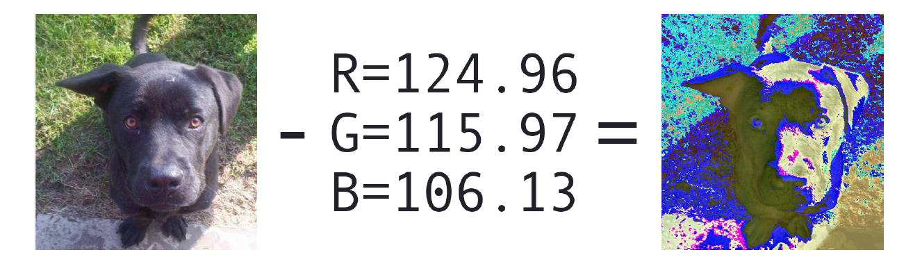
1.零均值化(数据归一化的一种形式):将输入的图像减去数据集中的红色、绿色和蓝色三个颜色通道的平均值。
2.patch Preprocessing:在训练过程中,随机从原始图像中提取MxN大小特征图像。
3.过采样:在测试时,对输入图像的五个区域(四个角+中心区域)进行裁剪并且对剪裁之后的特征图像进行水平翻转,总共会得到10张特征图像。
其中需要注意的是,过采样方法我们只在测试数据集上使用,通过过采样方法,我们得到10张特征图像,然后模型会对每一张图像进行预测,得到10个结果,最后通过投票或者平均计算得到最终的结果,从结果中我们将看到该方法有助于提高分类准确度。
零均值
在第9节 中,我们在将图像数据集转换为HDF5格式的过程中,计算了训练数据集中图像的红、绿、蓝三个颜色通道的平均值,之后,我们对每一张输入图像都减去对应通道平均值,这个过程我们称为数据归一化。即给定输入图像I及其对应R、G、B通道值,则可以通过:
R = R - μ R \mu_{R} μ R
G = G - μ G \mu_{G} μ G
B = B - μ B \mu_{B} μ B
其中,μ R , μ G , μ B \mu_{R},\mu_{G},\mu_{B} μ R , μ G , μ B
图10.1 左:原始图像,右:均值处理之后的图像
在代码实现零均值过程之前,我们首先看看整个项目结构,即:
1
2
3
4
5
6
7
8
9
10
11
--- pyimagesearch | |--- __init__.py | |--- callbacks | |--- nn | |--- preprocessing | | |--- __init__.py | | |--- aspectawarepreprocessor.py | | |--- imagetoarraypreprocessor.py | | |--- meanpreprocessor.py | | |--- simplepreprocessor.py | |--- utils
在pyimagesearch项目中的preprocessing子模块中新建一个meanpreprocessor.py ,并写入以下代码:
1 2 3 4 5 6 7 8 import cv2class MeanPreprocessor : def __init__ (self,rMean,gMean,bMean ): self .rMean = rMean self .gMean = gMean self .bMean = bMean
其中,三个参数分别是对应的三个颜色通道的均值。
接下来,让我们定义预处理函数:
1
2
3
4
5
6
7
8
def preprocess (self,image ): (B,G,R) = cv2.split(image.astype("float32" )) R -= self .rMean G -= self .gMean B -= self .bMean return cv2.merge([B,G,R])
需要注意的是cv2.split函数是把图像划分成对应的B,G,R,而不是R,G,B。
patch Preprocessing
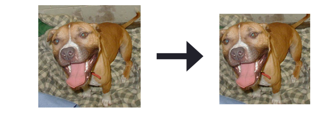
PatchPreprocessor类主要是在训练过程中随机抽取原始图像的MxN大小的特征图像。当输入的图像的维度比CNN模型要求的维度大时,我们就需要使用到patch Preprocessing——这是降低过拟合的常用技术,因此也是一种正则化形式。我们不会在训练过程中使用整个图像,而是随机裁剪其中的一部分,并将其传递给网络(关于裁剪预处理的示例,请参见图10.2)。
图10.2 左:原始256x256图像, 右:随机裁剪之后的227x227图像
使用随机裁剪方法意味着网络永远不会看到完全相同的图像(除非随机发生),类似于数据增强。在[第9节](http://lonepatient.top/2018/04/09/Deep_Learning_For_Computer_Vision_With_Python_PB_09.html)中,我们将kaggle上猫狗比赛数据集保存为HDF5数据集,其中原始数据的大小为256x256。然而,我们将在本章后面实现的AlexNet架构只能接受大小为227x227的图像。
那么,该如何处理?直接应用simplepreprocessor将每个256x256图像调整到227x227?从图10.2中,我们看到这样会损失图像信息,合理的做法是在训练过程中将256x256图像中随机裁剪出一个227x227特征图像——事实上,一方面类似于数据增强,另一方面这个过程正是Krizhevsky等人在ImageNet数据集中训练AlexNet的方式。
与其他图像预处理程序一样,patchpreprocessor预处理代码放在pyimagesearch的预处理子模块中,即:
1
2
3
4
5
6
7
8
9
10
11
12
--- pyimagesearch | |--- __init__.py | |--- callbacks | |--- nn | |--- preprocessing | | |--- __init__.py | | |--- aspectawarepreprocessor.py | | |--- imagetoarraypreprocessor.py | | |--- meanpreprocessor.py | | |--- patchpreprocessor.py | | |--- simplepreprocessor.py | |--- utils
打开patchpreprocessor.py ,并写入以下代码:
1 2 3 4 5 6 7 from sklearn.feature_extraction.image import extract_patches_2dclass PatchPreprocessor : def __init__ (self,width,height ): self .width = width self .height = height
其中,width和heigh分别表示裁剪后的图像宽度和高度。
接下来,定义预处理函数:
1
2
3
4
def preprocess (self,image ): return extract_patches_2d(image,(self .height,self .width), max_patches = 1 )[0 ]
给定需要返回的图像的宽度和高度,我们使用scikit-learn库的extract_patches_2d函数从原始图像中随机裁剪出指定大小的图像,其中参数max_patch =1,表明我们只需要输入图像中的一个随机patch。
PatchPreprocessor类看起来代码并不是很多,但它实际上是一种非常有效的方法,类似于数据增强,一定程度上可以降低过拟合。一般在训练过程中使用PatchPreprocessor。
随机裁剪
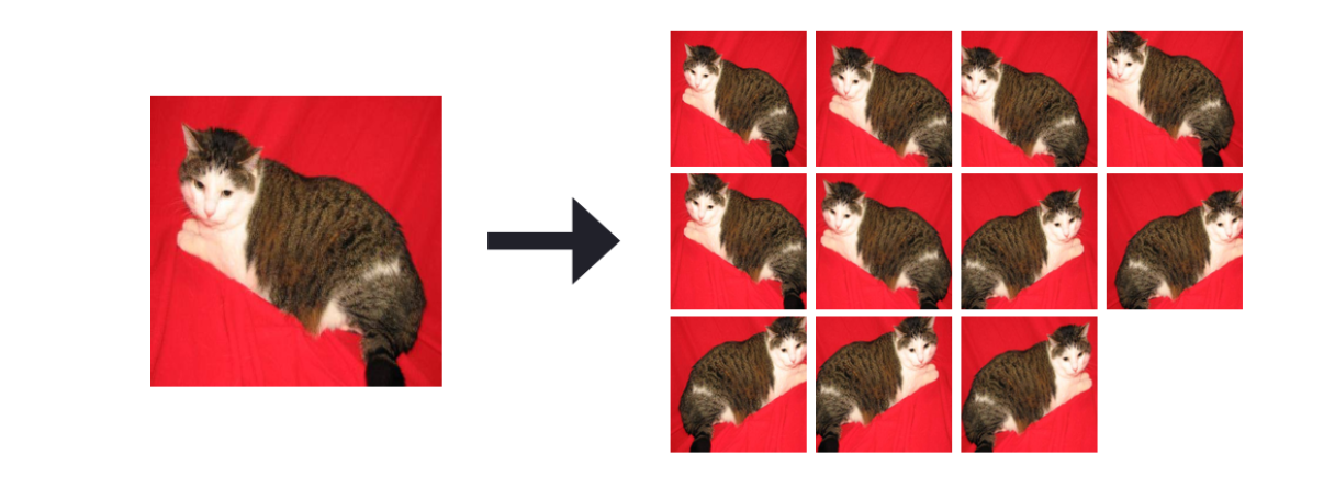
接下来,我们定义一个CropPreprocessor。在CNN的评估阶段,我们对输入图像的四个角+中心区域进行裁剪,然后进行相应的水平翻转,最后会产生10个样本(图10.3)。
图10.3 左: 原始256x256图像,右:裁剪得到的10张227x227图像
CNN模型将对这10个测试样本进行预测,产生10个结果,最后通过投票或者计算平均得到最终结果。利用这种过采样的方法,往往会增加1- 2%的分类准确率(在某些情况下,甚至更高)。
CropPreprocessor类也将存在于pyimagesearch的preprocessing子模块中:
1
2
3
4
5
6
7
8
9
10
11
12
13
--- pyimagesearch | |--- __init__.py | |--- callbacks | |--- nn | |--- preprocessing | | |--- __init__.py | | |--- aspectawarepreprocessor.py | | |--- croppreprocessor.py | | |--- imagetoarraypreprocessor.py | | |--- meanpreprocessor.py | | |--- patchpreprocessor.py | | |--- simplepreprocessor.py | |--- utils
打开croppreprocessor.py文件,写入以下代码:
1 2 3 4 5 6 7 8 9 10 import numpy as npimport cv2class GropPreprocessor : def __init__ (self,width,height,horiz = True ,inter=cv2.INTER_AREA ): self .width = width self .heiggt = height self .horiz = horiz self .inter = inter
其中,参数分别为:
width: 输出的图像宽度
heigh:输出的图像高度
horiz:是否进行水平翻转,默认为True
inter:openCV中用于调整大小的插值算法
定义预处理方法:
1
2
3
4
5
6
7
8
9
10
11
12
13
14
15
def preprocess (self,image ): crops = [] (h,w) = image.shape[:2 ] coords = [ [0 ,0 ,self .width,self .height], [w - self .width,0 ,w,self .height], [w - self .width,h - self .height,w,h], [0 ,h - self .height,self .width,h] ] dW = int (0.5 * (w - self .width)) dH = int (0.5 * (h - self .height)) coords.append([dW,dH,w - dW,h - dH])
其中预处理主函数只有一个参数,就是输入的图像,然后我们计算四个角(左上角、右上角、右下角、左下角)的坐标(x,y)以及中心坐标。并提取对应的部分图像:
1
2
3
4
5
6
7
8
9
10
11
12
for (startX,startY,endX,endY) in coords: crop = image[startY:endY,startX:endX] crop = cv2.resize(crop,(self .width,self .height), interpolation = self .inter) crops.append(crop) if self .horiz: mirrors = [cv2.flip(x,1 ) for x in crops] crops.extend(mirrors) return np.array(crops)
由于提取的图像大小会与目标大小存在1左右的差别,因此,我们进行调整大小。通过水平翻转,我们可以得到10张特征图像。
HDF5数据集生成器
在训练模型之前,我们首先需要定义一个类,用于从HDF5数据集中生成batch大小的图像数据和对应的标签。在第9节 中讨论了如何将保存在磁盘上的一组图像转换为HDF5数据集——但是我们如何将它们重新返回?
在pyimagesearch的io子模块中定义一个HDF5DatasetGenerator类:
1
2
3
4
5
6
7
8
9
10
--- pyimagesearch | |--- __init__.py | |--- callbacks | |--- io | | |--- __init__.py | | |--- hdf5datasetgenerator.py | | |--- hdf5datasetwriter.py | |--- nn | |--- preprocessing | |--- utils
之前训练模型时,所有图像数据集都可以加载到内存中,这样我们就可以依赖Keras生成器工具来生成batch大小的图像和相应的标签。但是,由于我们的数据集太大,无法全部加载到内存,所以我们需要自己实现一个针对HDF5数据集的生成器。
打开hdf5datasetgenerator.py文件,写入以下代码:
1 2 3 4 5 6 7 8 9 10 11 12 13 14 15 16 17 from keras.utils import np_utilsimport numpy as npimport h5pyclass HDF5DatasetGenerator : def __inti__ (self,dbPath,batchSize,preprocessors = None , aug = None ,binarize=True ,classes=2 ): self .batchSize = batchSize self .preprocessors = preprocessors self .aug = aug self .binarize = binarize self .classes = classes self .db = h5py.File(dbPath) self .numImages = self .db['labels' ].shape[0 ]
其中,参数分别为:
dbPath: HDF5数据集的路径
batchSize: batch数据量的大小
preprocessors:数据预处理列表,比如(MeanPreprocessor,ImageToArrayPreprocessor等等)。
aug: 默认为None,可以使用Keras中的ImageDataGenerator模块来进行数据增强。
binarize: 通常我们将类标签作为一个整数存储在HDF5数据集中,但是,如果我们使用categorical cross-entropy或者binary cross-entropy作为损失函数,那么我们需要把标签进行one-hot编码向量化——该参数主要说明是否进行二值化处理(默认为True)。
classes:类别个数,该数值决定了one-hot向量的shape
接下来,我们需要定义一个生成器函数,它负责在训练网络时将batch大小的图像和类标签传递给keras.fit_generator函数。
1
2
3
4
5
6
7
8
9
def generator (self,passes=np.inf ): epochs = 0 while epochs < passes: for i in np.arange(0 ,self .numImages,self .batchSize): images = self .db['images' ][i: i+self .batchSize] labels = self .db['labels' ][i: i+self .batchSize]
其中,passes为epochs的总数,一般而言,我们不用关心passes数值大小,因为在训练过程中,往往我们会指定训练的epoch个数,或者使用early stopping等等。所以默认为np.inf,即该循环会一直进行,直到:
1.模型训练达到终止条件。
2.手动停止(例如,ctrl + c)。
从hdf5数据集中提取数据之后,我们需要对数据进行预处理和标签one-hot编码:
1
2
3
4
5
6
7
8
9
10
if self .binarize: labels = np_utils.to_categorical(labels,self .calsses) if self .preprocessors is not None : proImages = [] for image in images: for p in self .preprocessors: image = p.preprocess(image) proImages.append(image) images = np.array(proImages)
同样也可以设置是否进行数据增强处理:
1
2
3
4
if self .aug is not None : (images,labels) = next (self .aug.flow(images, labels,batch_size = self .batchSize))
最后,我们将返回由图像和标签组成的二元祖数据,
1 2 3 4 5 6 yield (images,labels) epochs += 1 def close (self ): self .db.close()
整个HDF5数据集的生成器已经完成,在实际应用中,我们往往需要额外的工具来帮助我们快速地处理数据集,尤其是那些太大而无法加载到内存的数据集。后面,我们在开发深度学习项目或者实验时,HDF5DatasetGenerator将会加速我们处理数据的速度。
AlexNet
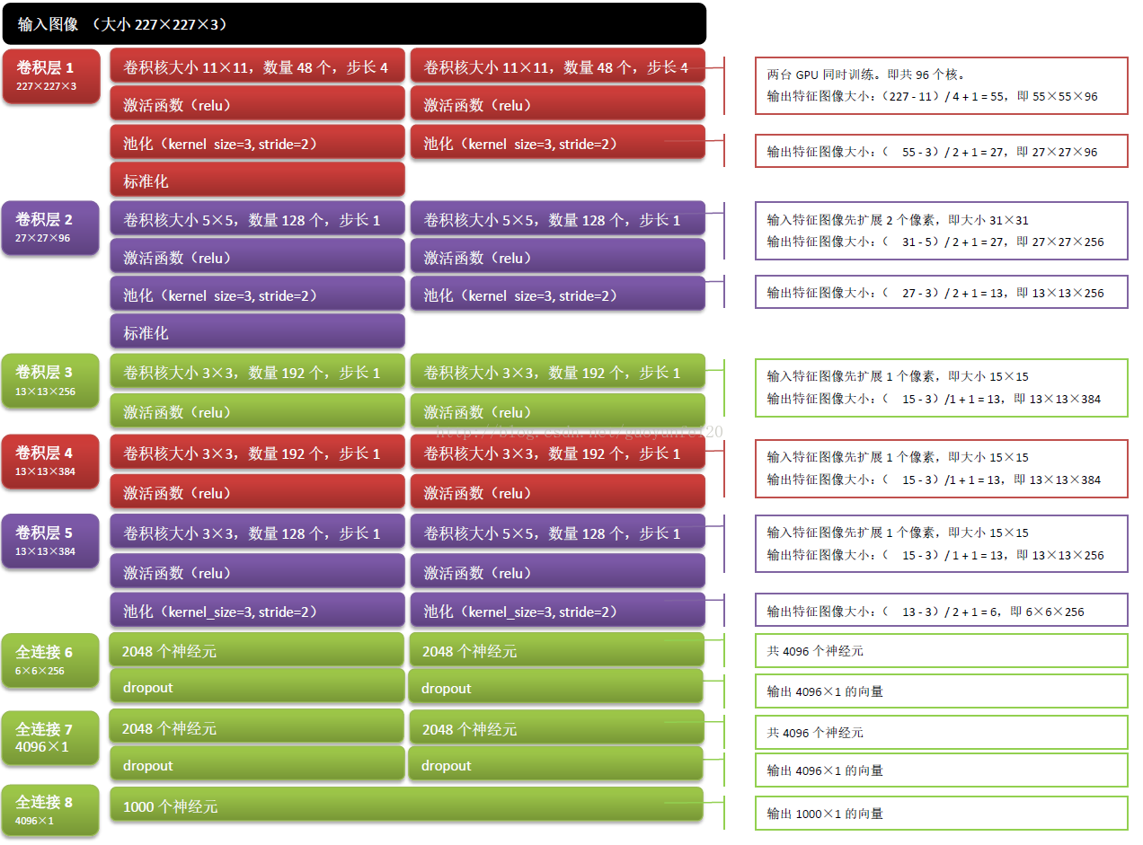
这部分,我们将实现Krizhevsky等人提出的具有开创性的AlexNet架构。完整的AlexNet网络架构如下图所示:
图10.4 AlexNet结构
为什么我们将输入图像的大小调整为227x227x3——这实际上是AlexNet架构要求的正确输入大小。实际上,Krizhevsky等人发表的原论文中使用的图像维度是224x224x3,但是,使用大小为11x1的卷积核遍历图像,会发现边界填充的结果是小数,这个显然是不对的,即(224-11) /4+1的结果是小数,通过推导实际上应该是227x227。
说明 :输出数据体在空间上的尺寸可以通过输入数据尺寸(W),卷积层中神经元的感受野尺寸(F),步长(S)和零填充的数量(P)的函数来计算,即数据体的空间尺寸为(W-F+2P)/s+1.
接下来,在pyimagesearch中nn的conv子模块中创建一个名为alexnet.py文件,如下目录结构:
1
2
3
4
5
6
7
8
9
10
11
12
--- pyimagesearch | |--- __init__.py | |--- callbacks | |--- io | |--- nn | | |--- __init__.py | | |--- conv | | | |--- __init__.py | | | |--- alexnet.py ... | |--- preprocessing | |--- utils
打开alexnet.py ,并写入以下代码:
1 2 3 4 5 6 7 8 9 10 11 12 from keras.models import Sequentialfrom keras.layers import BatchNormalizationfrom keras.layers import Conv2Dfrom keras.layers import MaxPooling2Dfrom keras.layers import Activationfrom keras.layers import Flattenfrom keras.layers import Dropoutfrom keras.layers import Densefrom keras.regularizers import l2from keras import backend as K
从加载的模块中可以看出,我们使用了BN和l2模块。AlexNet原文中使用的标准化是LRN(局部响应归一化),在实现中,我们使用更高级的BN算法,另外为了防止过拟合,我们将会卷积层和FC使用l2正则化。
下面,定义AlexNet结构:
1
2
3
4
5
6
7
8
9
10
11
class AlexNet : @staticmethod def build (width,height,depth,classes,reg=0.0002 ): model = Sequential() inputShape = (height,width,depth) chanDim = -1 if K.image_data_format() == "channels_first" : inputShape = (depth,height,width) chanDim = 1
其中:
width:输入图像的宽度
height:输入图像的高度
depth:输入图像的通道数,彩色为3,灰色为1
classes:类别总数
reg:正则化系数,对于较大、较深的网络,应用正则化有助于降低过拟合,同时提高准确度
接下来,我们构建模型的主体部分。首先,定义网络中的第一个CONV => RELU =>POOL 模块:
1 2 3 4 5 6 7 model.add(Conv2D(96 ,(11 ,11 ),strides=(4 ,4 ),input_shape=inputShape, padding='same' ,kernel_regularizer=l2(reg))) model.add(Activation('relu' )) model.add(BatchNormalization(axis = chanDim)) model.add(MaxPooling2D(pool_size = (3 ,3 ),strides=(2 ,2 ))) model.add(Dropout(0.25 ))
第一个CONV层有96个过滤器,每个过滤器大小为11x11,平移步长为4,激活函数为RELU,并且对卷积层使用了l2正则化(l2正则化后面会一直应用在CONV层和FC层)。
从图10.4,可以看出卷积层之后,是标准化操作,原文论文中使用的标准化为LRN,这里我们使用更加高级的BN层。标准化之后,是MaxPooling2D层,pool层可以降低特征图像维度,并减少参数量。最后,我们还增加了dropout层,进一步降低过拟合。
下面,我们定义第二个block,主要是CONV => RELU => POOL,类似于与第一个block,一共有256个过滤器,每一个过滤器的大小为5x5,平移步长为1:
1 2 3 4 5 6 7 model.add(Conv2D(256 ,(5 ,5 ),padding='same' , kernel_regularizer=l2(reg))) model.add(Activation('relu' )) model.add(BatchNormalization(axis=chanDim)) model.add(MaxPooling2D(pool_size=(3 ,3 ),strides(2 ,2 ))) model.add(Dropout(0.25 ))
定义第三个block,第三个block中叠加了多个CONV层,将学习到更深层次且丰富的特征:
1 2 3 4 5 6 7 8 9 10 11 12 13 14 15 model.add(Conv2D(384 ,(3 ,3 ),padding='same' , kernel_regularizer=l2(reg))) model.add(Activation('relu' )) model.add(BatchNormalization(axis = chanDim)) model.add(Conv2D(384 ,(3 ,3 ),padding='same' , kernel_regularizer=l2(reg))) model.add(Activation('relu' )) model.add(BatchNormalization(axis=chanDim)) model.add(Conv2D(256 ,(3 ,3 ),padding='same' , kernel_regularizer=l2(reg))) model.add(Activation('relu' )) model.add(BatchNormalization(axis = chanDim)) model.add(MaxPooling2D(pool_size=(3 ,3 ),strides=(2 ,2 )) model.add(Dropout(0.25 ))
前两个CONV层主要是由384个大小为3x3的过滤器组成,而第三个CONV由256个大小为3x3的过滤器组成,步长全部为1。
接着,我们拼接两个全连接层,每个全连接层都由4096神经元组成:
1 2 3 4 5 6 7 8 9 10 11 12 13 model.add(Flatten()) model.add(Dense(4096 ,kernel_regularizer=l2(reg))) model.add(Activation('relu' )) model.add(BatchNormalization(axis = chanDim)) model.add(Dropout(0.5 )) model.add(Dense(4096 ,kernel_regularizer=l2(reg))) model.add(Activation('relu' )) model.add(BatchNormalization(axis = chanDim)) model.add(Dropout(0.5 ))
在全连接FC层之后,紧接这BN层和Dropout层(一个较大的概率值,比如0.5)。
最后,我们定义一个softmax分类器,并将模型结果返回给调用函数:
1 2 3 4 5 6 model.add(Dense(classes,kernel_regularizer=l2(reg))) model.add(Activation('softmax' )) return model
从整个构建AlexNet网络架构过程中可以看到,我们完成是按照图10.1所示的体系结构进行编写代码,你会发现实现AlexNet模型是一个相当简单的过程。
训练猫狗数据集
前面我们已经定义好AlexNet模型架构,接下来,我们开始训练猫狗数据集,新建一个名为train_alexnet.py,写入以下代码:
1 2 3 4 5 6 7 8 9 10 11 12 13 14 15 16 import matplotlibmatplotlib.use('Agg' ) from config import dogs_vs_cats_config as configfrom pyimagesearch.preprocessing import imagetoarraypreprocessor as IAPfrom pyimagesearch.preprocessing import simplespreprocessor as SPfrom pyimagesearch.preprocessing import patchpreprocessor as PPfrom pyimagesearch.preprocessing import meanpreprocessor as MPfrom pyimagesearch.callbacks import trainingmonitor as TMfrom pyimagesearch.io import hdf5datasetgenerator as HDFfrom pyimagesearch.nn.conv import alexnetfrom keras.preprocessing.image import ImageDataGeneratorfrom keras.optimizers import Adamimport jsonimport os
在大多数计算机视觉任务中,我们都建议使用数据增强技术,因此,我们对猫狗数据集进行数据增强处理:
1 2 3 4 5 aug = ImageDataGenerator(rotation_range = 20 ,zoom_range = 0.15 , width_shift_range = 0.2 ,height_shift_range = 0.2 , shear_range=0.15 ,horizontal_flip=True , fill_mode='nearest' )
初始化数据预处理模块:
1 2 3 4 5 6 7 means = json.loads(open (config.DATASET_MEAN).read()) sp = SP.SimplePreprocessor(227 ,227 ) pp = PP.PatchPreprocessor(227 ,227 ) mp = MP.MeanPreprocessor(means['R' ],means['G' ],means['B' ]) iap = IAP.ImageToArrayPreprocessor()
这里,我们初始化了三个预处理方法,其中:
means:RGB颜色通道平均值数据
sp:将图像大小调整到227x227,该函数主要对验证数据集
pp:随机从原始256x256图像中裁剪出227x227大小特征图像,该函数主要是针对训练数据集
mp: 零均值化,将特征图像减去对应通道的平均值
iap: 将特征图像转换为keras支持的数组形式
初始化训练数据集和验证数据集生成器:
1 2 3 trainGen = HDF.HDF5DatasetGenerator(dbPath=config.TRAIN_HDF5,batchSize=128 ,aug=aug,preprocessors= [pp,mp,iap],classes = 2 ) valGen = HDF.HDF5DatasetGenerator(config.VAL_HDF5,128 ,preprocessors=[sp,mp,iap],classes =2 )
在这里需要注意 训练数据集生成器和验证数据集生成器的参数值区别。
初始化Adam优化器和AlexNet模型:
1 2 3 4 5 6 7 8 9 10 11 print ("[INFO] compiling model..." )opt = Adam(lr=1e-3 ) model = alexnet.AlexNet.build(width=227 ,height=227 ,depth=3 , classes=2 ,reg=0.0002 ) model.compile (loss = 'binary_crossentropy' ,optimizer=opt, metrics = ['accuracy' ]) path = os.path.sep.join([config.OUTPUT_PATH,"{}.png" .format (os.getpid())]) callbacks = [TM.TrainingMonitor(path)]
在第7节 中我们学习了几种自适应学习率优化算法,本节中,我们将使用Adam优化算法(默认学习率为0.001)。选择Adam(而不是SGD),主要由于:
1.尝试更高级的优化算法。
2.针对该分类任务,Adam比SGD表现得更好。
前面,我们分析了AlexNet模型输入的图像的shape应为(227,227,3)。另外,对于一般二元分类问题常用的loss函数为binary cross-entropy,多分类问题常用的loss函数为categorical cross-entropy,因此,这里我们使用的loss函数为binary cross-entropy。callbacks回调参数主要是为了方便在网络进行训练时监视其性能。
训练网络:
1 2 3 4 5 6 7 8 9 10 model.fit_generator( trainGen.generator(), steps_per_epoch = trainGen.numImages // 128 , validation_data = valGen.generator(), validation_steps = valGen.numImages // 128 , epochs = 75 , max_queue_size = 128 * 2 , callbacks = callbacks, verbose = 1 )
我们的数据是从生成器返回的,因此,我们这里使用的是.fit_generator方法
训练完模型之后,我们将得到的模型保存在磁盘中:
1 2 3 4 5 6 7 print ("[INFO] serializing model ...." )model.save(config.MODEL_PATH,overwrite = True ) trainGen.close() valGen.close()
上面,我们完成从数据获取、数据预处理和训练模型,接下来,执行以下命令:
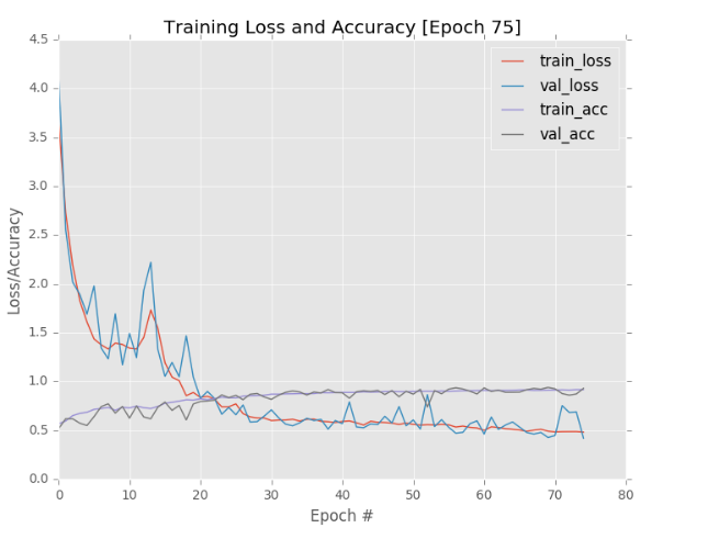
1
2
3
4
5
6
7
8
$ python train_alexnet.py Epoch 73/75 415s - loss: 0.4862 - acc: 0.9126 - val_loss: 0.6826 - val_acc: 0.8602 Epoch 74/75 408s - loss: 0.4865 - acc: 0.9166 - val_loss: 0.6894 - val_acc: 0.8721 Epoch 75/75 401s - loss: 0.4813 - acc: 0.9166 - val_loss: 0.4195 - val_acc: 0.9297 [INFO] serializing model...
当75次训练迭代结束后,我们可以得到如图10.5的训练和验证的loss/accuracy曲线图。总的来说,我们可以看到训练次数和准确率之间具有一定的相关性,另外,从图中我们可以看到验证loss并没还稳定下来,那么我们可以加大epochs次数,当然我们也可以通过应用一些学习率衰减方法,使得只在75次迭代中,验证loss趋向于稳定。从结果中,我们可以看到验证集的精度达到了92.97%。
图10.5 AlexNet模型性能曲线
接下来,我们对测试集做两次实验,即:
1.直接模型对原始测试集进行预测,并查看结果
2.先对测试集进行过采样方法,然后使用对采样得到数据进行预测,并查看结果
你将从结果中看到,对测试集使用过采样方法,精度会提高了1-3%左右。
性能评估
新建一个名为crop_accuracy.py的文件,如以下结构:
1
2
3
4
5
6
7
8
--- dogs_vs_cats | |--- config | |--- build_dogs_vs_cats.py | |--- crop_accuracy.py | |--- extract_features.py | |--- train_alexnet.py | |--- train_model.py | |--- output
打开crop_accuracy.py,并写入以下代码:
1 2 3 4 5 6 7 8 9 10 11 12 13 from config import dogs_vs_cats_config as configfrom pyimagesearch.preprocessing import imagetoarraypreprocessor as IAPfrom pyimagesearch.preprocessing import simplespreprocessor as SPfrom pyimagesearch.preprocessing import patchpreprocessor as PPfrom pyimagesearch.preprocessing import meanpreprocessor as MPfrom pyimagesearch.preprocessing import croppreprocessor as CPfrom pyimagesearch.io import hdf5datasetgenerator as HDFfrom pyimagesearch.utils.ranked import rank5_accuracyfrom keras.models import load_modelimport numpy as npimport progressbarimport json
从磁盘中加载RGB均值数据,并初始化图像预处理和加载预先训练好的AlexNet网络:
1 2 3 4 5 6 7 8 9 10 11 12 means = json.loads(open (config.DATASET_MEAN).read()) sp = SP.SimplePreprocessor(227 ,227 ) mp = MP.MeanPreprocessor(means['R' ],means['G' ],means['B' ]) cp = CP.CropPreprocessor(227 ,227 ) iap = IAP.ImageToArrayPreprocessor() print ("[INFO] loading model ..." )model = load_model(config.MODEL_PATH)
在应用过采样方法之前,我们先在测试集上获得一个baseline,即模型对原始的测试图像进行预测:
1 2 3 4 5 6 7 8 9 10 11 12 print ("[INFO] predicting on test data (no crops)..." )testGen = HDF.HDF5DatasetGenerator(config.TEST_HDF5,64 , preprocessors = [sp,mp,iap], classes = 2 ) predictions = model.predict_generator(testGen.generator(), steps = testGen.numImages // 64 , max_queue_size = 64 * 2 ) (rank1,_) = rank5_accuracy(predictions,testGen.db['labels' ]) print ("[INFO] rank-1: {:.2f}%" .format (rank1 * 100 ))testGen.close()
猫狗数据集是一个二分类问题,因此我们只关心rank-1准确度,如果计算rank-5准确度,那么会得到100%的rank-5准确度,这是无意义的。
接下来,我们对测试集数据进行过采样:
1 2 3 4 5 6 7 8 9 10 testGen = HDF.HDF5DatasetGenerator(config.TEST_HDF5,64 , preprocessors = [mp],classes = 2 ) predictions = [] widgets = ['Evaluating: ' ,progressbar.Percentage()," " , progressbar.Bar()," " ,progressbar.ETA()] pbar = progressbar.ProgressBar(maxval = testGen.numImages // 64 , widgets=widgets).start()
遍历每一张图像,并进行10-cropping方法,得到10张特征图像:
1 2 3 4 5 6 7 8 9 10 11 12 for (i,(images,labels)) in enumerate (testGen.generator(passes=1 )): for image in images: crops = cp.preprocess(image) crops = np.array([iap.preprocess(c) for c in crops], dtype = 'float32' ) pred = model.predict(crops) predictions.append(pred.mean(axis = 0 )) pbar.update(i)
训练时候,一般我们会设置HDF5DatasetGenerator为永久循环,直到满足一定条件后自动停止(通常在训练时设置最大的迭代次数)。但是,在测试过程中,我们只需循环一次,因此,passes =1。
对每个输入图像进行过采样处理——在原始256x256图像的基础上通过裁剪得到为10个227x227图像的数组,然后模型对每一个样本进行预测,最后计算平均值作为最终结果。
计算rank-1准确度:
1 2 3 4 5 6 pbar.finish() print ("[INFO] predicting on test data (with crops)...." )(rank1,_) = rank5_accuracy(predictions,testGen.db['labels' ]) print ("[INFO'] rank-1: {:.2f}%" .format (rank1 * 100 ))testGen.close()
执行以下命令,查看性能结果:
1
2
3
4
5
6
7
$ python crop_accuracy.py [INFO] loading model... [INFO] predicting on test data (no crops)... [INFO] rank-1: 92.60% Evaluating: 100% |####################################| Time: 0:01:12 [INFO] predicting on test data (with crops)... [INFO] rank-1: 94.00%
如结果所示,第1个实验中,模型在测试集上的准确率达到了92.60%。但是,在第2个实验中,通过10-cropping的过采样方法,我们能够将分类准确率提高到94.00%,增加了1.4%。简单的一个操作,让精度提高了1-3%左右。
Top30
如果你观察了Kaggle猫狗比赛的排行榜,你会发现,要想进入前30名,我们差不多需要96.69%的准确率,而我们目前的方法是无法达到的。那么该如何提高呢?
我们主要使用转移学习——通过特征提取。虽然ImageNet数据集包含1000个对象类别,但其中很大一部分包含了狗的种类和猫的种类。说明在ImageNet上训练的网络不仅能告诉你一个图片是狗还是猫,而且还能告诉你这个动物是什么品种。鉴于在ImageNet上训练的网络具有区分这些细粒度特征的能力,我们可能会想到直接对预先训练好的网络中提取出来的特征向量训练一个常见的机器学习模型,很可能会获得更好的结果。
接下来,我们来实现这个过程,我们首先从训练好的ResNet模型中提取特征,然后对这些特征向量训练逻辑回归分类器。
提取特征-ResNet
在第3节 中,我们讨论了特征提取的详细内容,这里,就不做详细的描述。我们新建一个extract_features.py,并写入一下代码:
1 2 3 4 5 6 7 8 9 10 11 12 13 14 from keras.applications import ResNet50from keras.applications import imagenet_utilsfrom keras.preprocessing.image import img_to_arrayfrom keras.preprocessing.image import load_imgfrom sklearn.preprocessing import LabelEncoderfrom pyimagesearch.io import hdf5datasetwriter as HDFfrom imutils import pathsimport numpy as npimport progressbarimport argparseimport randomimport os
使用keras加载预先训练好的ResNet50模型,若本地没有模型文件,则keras会自动进行下载。
解析命令行参数:
1 2 3 4 5 6 7 8 9 10 11 12 13 ap = argparse.ArgumentParser() ap.add_argument('-d' ,"--dataset" ,required = True , help = 'path to input dataset' ) ap.add_argument("-0" ,'--output' ,required = True , help = 'path ot output hdf5 file' ) ap.add_argument('-b' ,'--batch_size' ,type = int ,default = 16 , help ='batch size of images to ba passed through network' ) ap.add_argument('-s' ,'--buffer_size' ,type =int ,default=1000 , help = 'size of feature extraction buffer' ) args = vars (ap.parse_args()) bs = args['batch_size' ]
其中:
datset:输入数据的路径
output: 输出路径
batch_size: batch数量的大小,默认为16
buffer_size: 默认1000,每1000次进行一次 操作
从磁盘中读取数据集并提取相应的标签数据:
1
2
3
4
5
6
7
8
9
print ("[INFO] loading images..." )imagePaths = list (paths.list_images(args['dataset' ])) random.shuffle(imagePaths) labels = [p.split(os.path.sep)[-1 ].split("." )[0 ] for p in imagePaths] le = LabelEncoder() labels = le.fit_transform(labels)
可以磁盘中加载预训练的ResNet50模型权重(不包括FC层):
1 2 3 4 print ("[INFO] loading network..." )model = ResNet50(weights = 'imagenet' ,include_top=False )
为了将从ResNet50提取的特征数据存储到磁盘,我们需要实例化aHDF5DatasetWriter对象:
1 2 3 4 5 ResNet50的最后一个average pooling层的维度是2048 dataset = HDF.HDF5DatasetWriter((len (imagePaths),2048 ), args['output' ],dataKey='feature' ,buffSize=args['buffer_size' ]) dataset.storeClassLabels(le.classes_)
初始化progressbar,以便跟踪特征提取过程:
1 2 3 4 5 widgets = ['Extracting Features: ' ,progressbar.Percentage(),' ' , progressbar.Bar(),' ' ,progressbar.ETA()] pbar = progressbar.ProgressBar(maxval = len (imagePaths), widgets = widgets).start()
使用CNN从数据集中提取特征与在第3章中一样。首先,我们对图像路径数据进行批量循环:
1 2 3 4 5 6 for i in np.arange(0 ,len (imagePaths),bs): batchPaths = imagePaths[i:i+bs] batchLabels = labels[i:i+bs] batchImages = []
然后对每张图像进行预处理:
1 2 3 4 5 6 7 8 9 for (j,imagePath) in enumerate (batchPaths): image = load_img(imagePath,target_size = (224 ,224 )) image = img_to_array(image) image = np.expand_dims(image,axis = 0 ) image = imagenet_utils.preprocess_input(image) batchImages.append(image)
从ResNet50的最后一个池化层中提取特征数据:
1
2
3
4
5
batchImages = np.vstack(batchImages) features = model.predict(batchImages,batch_size=bs) features = features.reshape((features.shape[0 ],2048 ))
然后将这些提取出来的特征向量保存到HDF5数据集中:
1 2 3 4 5 6 dataset.add(features,batchLabels) pbar.update(i) dataset.close() pbar.finish()
执行以下命令,完成整个特征提取步骤:
1
2
3
4
5
$ python extract_features.py --dataset ../datasets/kaggle_dogs_vs_cats/train \ --output ../datasets/kaggle_dogs_vs_cats/hdf5/features.hdf5 [INFO] loading images... [INFO] loading network... Extracting Features: 100% |####################################| Time: 0:06:18
执行完命令后,查看输出目录:
1
2
$ ls -l ../datasets/kaggle_dogs_vs_cats/hdf5/features.hdf5-rw-rw-r-- adrian 409806272 Jun 3 07:17 output/dogs_vs_cats_features.hdf5
基于这些特征向量,我们将训练一个逻辑回归分类器。
逻辑回归
新建一个名为train_model.py文件,并写入以下代码:
1 2 3 4 5 6 7 8 from sklearn.linear_model import LogisticRegressionfrom sklearn.model_selection import GridSearchCVfrom sklearn.metrics import classification_reportfrom sklearn.metrics import accuracy_scoreimport argparseimport pickleimport h5py
解析命令行参数:
1 2 3 4 5 6 7 8 9 ap = argparse.ArgumentParser() ap.add_argument("-d" ,"--db" ,required = True , help = 'path HDF5 datasetbase' ) ap.add_argument('-m' ,'--model' ,required=True , help ='path to output model' ) ap.add_argument('-j' ,'--jobs' ,type =int ,default=-1 , help = '# of jobs to run when tuning hyperparameters' ) args = vars (ap.parse_args())
其中:
db: HDF5数据集的路径
model:模型输出路径
jobs:资源使用数,默认值为-1,即使用全部资源
从HDF5数据集中读取数据,并进行数据划分——75%的数据用于训练,25%用于测试:
1 2 3 db = h5py.File(args['db' ],'r' ) i = int (db['labels' ].shape[0 ] * 0.75 )
逻辑回归只有一个超参数需要调整——正则化系数C,我们使用网格搜索进行调参:
1
2
3
4
5
6
7
8
print ("[INFO] tuning hyperparameters..." )params = {"C" :[0.0001 ,0.001 ,0.01 ,0.1 ,1.0 ]} model = GridSearchCV(LogisticRegression(),params,cv =3 , n_jobs = args['jobs' ]) model.fit(db['feature' ][:i],db['labels' ][:i]) print ('[INFO] best hyperparameters: {}' .format (model.best_params_))
一旦我们找到C的最佳选择,我们就可以为测试集生成分类报告:
1 2 3 4 5 6 7 8 print ('[INFO] evaluating...' )preds = model.predict(db['feature' ][i:]) print (classification_report(db['labels' ][i:],preds, target_names = db['label_names' ])) acc = accuracy_score(db['labels' ][i:],preds) print ('[INFO] score: {}' .format (acc))
将训练好的logistics regression模型保存到磁盘:
1 2 3 4 5 6 print ('[INFO] saving model...' )with open (args['model' ],'wb' ) as fw: fw.write(pickle.dumps(model.best_estimator_)) db.close()
运行下面命令,完成整个提取特征和训练模型过程:
1
2
3
4
5
6
7
8
9
10
11
12
13
14
python train_model.py --db ../datasets/kaggle_dogs_vs_cats/hdf5/features.hdf5 \ --model dogs_vs_cats.pickle [INFO] tuning hyperparameters... [INFO] best hyperparameters: {’C’: 0.001} [INFO] evaluating... precision recall f1-score support cat 0.99 0.99 0.99 3115 dog 0.99 0.99 0.99 3135 avg / total 0.99 0.99 0.99 6250 [INFO] score: 0.986 [INFO] saving model...
从输出结果中可以看到的,我们通过迁移学习的方法获得了惊人的准确率98.69%,这足以让我们在Kaggle排行榜上占据第二。
Summary
在本章中,我们深入研究了Kaggle猫狗数据集,并对数据集做了两组不同的实验且都获得了> 90%分类准确率:
1.从头训练一个AlexNet模型。
2.通过ResNet应用迁移学习。
我们使用简单的AlexNet模型结构,达到了94%的分类精度。而且我们是从头开始训练一个网络,这已经是一个相当不错的结果。另外我们还可以通过一些手段提高准确度:
1.获得更多的训练数据。
2.应用更高级的数据增强方法。
3.加深网络。
然而,我们获得的94%精度还不足以进入前25名,更不用说前5名了。因此,为了获得前五名的位置,我们通过特征提取进行迁移学习——从ImageNet数据集训练好的ResNet50提取特征,因为ImageNet包含了许多狗和猫的例子,参考第8节内容 ,我们可以看到该挑战任务很适合使用迁移学习。正如我们的结果所显示的,我们获得98.69%的分类准确率,高到足以在排行榜上位居第二。
本文完整代码:github