超参数优化是实现模型性能最大化的重要步骤。为此大神们专门开发了几个Python包。scikitt -learn提供了一些选项,GridSearchCV和RandomizedSearchCV是两个比较流行的选项。在scikitt之外,Optunity、Spearmint和hyperopt包都是为优化设计的。在这篇文章中,我将重点介绍hyperopt软件包,它提供了能够超越随机搜索的算法,并且可以找到与网格搜索相媲美的结果,同时也能找到更少的模型。
接口说明
具体的详细文档: http://www.coxlab.org/pdfs/2013_bergstra_hyperopt.pdf
fmin接口:需要定义一个概率分布,确保能在变化的超参中找到一个可信的值。就像scipy中的optimize.minimize借口。因此需要我们提供一个优化的目标函数。很多优化算法都要假设在一个向量空间里面搜索最佳值,hyperopt可以对搜索空间进一步细化,比如说使用log话活着均匀分布随机获取之类。
hyperopt需要定义的主要有四个地方:
1.需要最小化的目标函数
2.优化所需要搜索的搜索空间
3.一个存放搜索过程计算结果的数据库(利用结果进行分析)
4.所使用的搜索算法
第一步 :定义目标函数
1
2
3
def q (args ): x,y = args return x ** 2 + y ** 2
第二步 :确定一个搜索空间
1
2
from hyperopt import hpspace = [hp.uniform("x" ,0 ,1 ),hp.normal("y" ,0 ,1 )]
接下来,对搜索空间的表达式进行说明。主要通过hyperopt .hp模块,比如:
1 fmin(q,space = hp.uniform(‘a’,0 ,1 ))
其中hp.uniform的第一位置表示标签,即“a”,在自定义空间中,每一个超参都必须有一个类似这样的标签。其他超参选择分布说明如下:
1
2
3
4
5
6
7
8
9
10
11
12
13
14
15
16
hp.choice(label,options): 返回options中的一个,因此options应该是一个列表或者元组。 hp.pchoice(label,p_options): 按照概率集p_options来选择option之间的一个,一次为(prob,option)形式 hp.uniform(label,low,high): 从low和high按照均匀分布产生数据 hp.quniform(label,low,high,q): 按照round (exp(uniform(low,high))/q)*q产生, hp.loguniform(label,low,high): 从exp(uniform(low,high)),当搜索空间限制在[exp(low),exp(high)]之间 hp.normal(label,mu,sigma): 从一个正态分布中产生数据,主要适用于无限制的变量 hp.lognormal(label, mu, sigma) : 从exp(normal(mu, sigma)).产生 ,该变量限制为正数 hp.randint(label, upper): 从[0 ,upper)中随机产生一个整数
第三步 :选择一个搜索算法
1
2
3
4
5
6
7
8
from hyperopt import hp, fmin, rand, tpe, space_evalbest = fmin(q, space, algo=rand.suggest) print bestprint space_eval(space, best)best = fmin(q, space, algo=tpe.suggest) print best
如果有多个需要优化的超参:则可以有不同写法,比如:
1
2
3
4
5
6
7
8
9
10
11
12
from hyperopt import hplist_space = [ hp.uniform(’a’, 0 , 1 ), hp.loguniform(’b’, 0 , 1 )] tuple_space = ( hp.uniform(’a’, 0 , 1 ), hp.loguniform(’b’, 0 , 1 )) dict_space = { ’a’: hp.uniform(’a’, 0 , 1 ), ’b’: hp.loguniform(’b’, 0 , 1 )}
可以使用hyperopt.pyll.stochastic从搜索空间中抽样,比如:
1
2
3
4
5
6
7
from hyperopt.pyll.stochastic import sampleprint sample(list_space)print sample(nested_space)
也可以在搜索空间定义表达式(这样的话就可以随意的构造你的搜索空间中的值,而不局限于在某一个向量空间中,如下:
1
2
3
4
5
6
7
8
9
10
11
12
13
14
15
16
17
18
19
20
from hyperopt.pyll import scopedef foo (x ): return str (x) * 3 expr_space = { ’a’: 1 + hp.uniform(’a’, 0 , 1 ), ’b’: scope.minimum(hp.loguniform(’b’, 0 , 1 ), 10 ), ’c’: scope.call(foo, args=(hp.randint(’c’, 5 ),)), } from hyperopt.pyll import scope@scope.define def foo (x ): return str (x) * 3 print foo(0 )expr_space = { 'a' : 1 + hp.uniform('a' , 0 , 1 ),'b' : scope.minimum(hp.loguniform('b' , 0 , 1 ), 10 ),'c' : scope.foo(hp.randint('cbase' , 5 )),}
接下来,主要看下几个常用的分类算法的使用方式:
1
2
3
4
5
6
7
8
9
10
11
12
13
14
15
16
17
18
from hyperopt import hpfrom hyperopt.pyll import scopefrom sklearn.naive_bayes import GaussianNBfrom sklearn.svm import SVCfrom sklearn.tree import DecisionTreeClassifier\as DTreescope.define(GaussianNB) scope.define(SVC) scope.define(DTree, name='DTree' ) C = hp.lognormal('svm_C' , 0 , 1 ) space = hp.pchoice('estimator' , [ (0.1 , scope.GaussianNB()), (0.2 , scope.SVC(C=C, kernel='linear' )), (0.3 , scope.SVC(C=C, kernel='rbf' ,width=hp.lognormal('svm_rbf_width' , 0 , 1 ))), (0.4 , scope.DTree(criterion=hp.choice('dtree_criterion' ,['gini' , 'entropy' ]), max_depth=hp.choice('dtree_max_depth' , [None , hp.qlognormal('dtree_max_depth_N' , 2 , 2 , 1 )])))])
第四步,存储搜索结果:trials结构,用法主要如下:
1
2
3
4
5
from hyperopt import (hp, fmin, space_eval,Trials)trials = Trials() best = fmin(q, space, trials=trials) print trials.trials
tid:整型,主要hitrial的识别(就是每一次调整的id)
定义的目标函数,需要返回的事字典的形式:如
1
2
3
4
5
6
7
8
9
10
11
12
13
14
15
import timefrom hyperopt import fmin, Trialsfrom hyperopt import STATUS_OK, STATUS_FAILdef f (x ): try : return {'loss' : x ** 2 , 'time' : time.time(), 'status' : STATUS_OK } except Exception, e: return {'status' : STATUS_FAIL, 'time' : time.time(), 'exception' : str (e)} trials = Trials() fmin(f, space=hp.uniform('x' , -10 , 10 ),trials=trials) print trials.trials[0 ]['results' ]
案例
主要使用xgboost,lightgbm,rf的用法
加载模块
1
2
3
4
5
6
7
8
9
import numpy as npimport pandas as pdfrom hyperopt import hp, tpefrom hyperopt.fmin import fminfrom sklearn.model_selection import cross_val_score, StratifiedKFoldfrom sklearn.ensemble import RandomForestClassifierfrom sklearn.metrics import make_scorerimport xgboost as xgbimport lightgbm as lgbm
数据集
1
2
3
df = pd.read_csv('../input/train.csv' ) X = df.drop(['id' , 'target' ], axis=1 ) Y = df['target' ]
评估指标
1
2
3
4
5
6
7
8
9
10
11
12
13
14
15
def gini (truth, predictions ): g = np.asarray(np.c_[truth, predictions, np.arange(len (truth)) ], dtype=np.float ) g = g[np.lexsort((g[:,2 ], -1 *g[:,1 ]))] gs = g[:,0 ].cumsum().sum () / g[:,0 ].sum () gs -= (len (truth) + 1 ) / 2. return gs / len (truth) def gini_xgb (predictions, truth ): truth = truth.get_label() return 'gini' , -1.0 * gini(truth, predictions) / gini(truth, truth) def gini_lgb (truth, predictions ): score = gini(truth, predictions) / gini(truth, truth) return 'gini' , score, True def gini_sklearn (truth, predictions ): return gini(truth, predictions) / gini(truth, truth) gini_scorer = make_scorer(gini_sklearn, greater_is_better=True , needs_proba=True )
Random Forest
在这一部分中,我们将使用hyperopt库来优化random forest classsifier。hyperopt库的目的与gridsearch类似,但是它没有对参数空间进行彻底的搜索,而是对一些精心选择的数据点进行评估,然后根据建模来推断出最优的解决方案。实际上,这意味着需要更少的迭代来找到一个好的解决方案。
随机森林的工作原理是通过许多决策树的平均预测来实现的——这个想法是,通过平均许多树,每棵树的错误都被解决了。每一种决策树都可能有点过分,通过平均它们的最终结果应该是好的。
调整的重要参数是:
树的数量(n_estimators)
1
2
3
4
5
6
7
8
9
10
11
12
13
14
def objective (params ): params = {'n_estimators' : int (params['n_estimators' ]), 'max_depth' : int (params['max_depth' ])} clf = RandomForestClassifier(n_jobs=4 , class_weight='balanced' , **params) score = cross_val_score(clf, X, Y, scoring=gini_scorer, cv=StratifiedKFold()).mean() print ("Gini {:.3f} params {}" .format (score, params)) return score space = { 'n_estimators' : hp.quniform('n_estimators' , 25 , 500 , 25 ), 'max_depth' : hp.quniform('max_depth' , 1 , 10 , 1 ) } best = fmin(fn=objective, space=space, algo=tpe.suggest, max_evals=10 )
1
2
3
4
5
6
7
8
9
10
Gini -0.218 params {'n_estimators': 50, 'max_depth': 1} Gini -0.243 params {'n_estimators': 175, 'max_depth': 4} Gini -0.237 params {'n_estimators': 475, 'max_depth': 3} Gini -0.252 params {'n_estimators': 450, 'max_depth': 6} Gini -0.236 params {'n_estimators': 300, 'max_depth': 3} Gini -0.251 params {'n_estimators': 225, 'max_depth': 6} Gini -0.237 params {'n_estimators': 450, 'max_depth': 3} Gini -0.254 params {'n_estimators': 400, 'max_depth': 8} Gini -0.243 params {'n_estimators': 450, 'max_depth': 4} Gini -0.252 params {'n_estimators': 450, 'max_depth': 6}
则最好的参数如下:
1 print ("Hyperopt estimated optimum {}" .format (best))
1 Hyperopt estimated optimum {'max_depth': 8.0, 'n_estimators': 400.0}
xgboost
类似于上面的调优,现在我们将使用hyperopt来优化xgboost参数!
XGBoost也是一种基于决策树的集合,但不同于随机森林。这些树不是平均的,而是增加的。决策树经过训练,可以纠正前几棵树的残差。这个想法是,许多小型决策树都经过了训练,每个决策树都添加了一些信息来提高总体预测。
我最初将树的数量固定在250,而学习速率是0.05(用一个快速的实验来确定)——然后我们可以为其他参数找到好的值。稍后我们可以重新迭代这个。
最重要的参数是:
树的数量(n_estimators)
学习速率-后树的影响较小(learning_rate)
树深度(max_depth)
gamma-过拟合参数。
colsample_bytree-减少过度拟合。
1
2
3
4
5
6
7
8
9
10
11
12
13
14
15
16
17
18
19
20
21
22
23
24
25
26
27
28
def objective (params ): params = { 'max_depth' : int (params['max_depth' ]), 'gamma' : "{:.3f}" .format (params['gamma' ]), 'colsample_bytree' : '{:.3f}' .format (params['colsample_bytree' ]), } clf = xgb.XGBClassifier( n_estimators=250 , learning_rate=0.05 , n_jobs=4 , **params ) score = cross_val_score(clf, X, Y, scoring=gini_scorer, cv=StratifiedKFold()).mean() print ("Gini {:.3f} params {}" .format (score, params)) return score space = { 'max_depth' : hp.quniform('max_depth' , 2 , 8 , 1 ), 'colsample_bytree' : hp.uniform('colsample_bytree' , 0.3 , 1.0 ), 'gamma' : hp.uniform('gamma' , 0.0 , 0.5 ), } best = fmin(fn=objective, space=space, algo=tpe.suggest, max_evals=10 )
1
2
3
4
5
6
7
8
9
10
Gini -0.268 params {'max_depth': 2, 'gamma': '0.221', 'colsample_bytree': '0.835'} Gini -0.268 params {'max_depth': 2, 'gamma': '0.231', 'colsample_bytree': '0.545'} Gini -0.271 params {'max_depth': 8, 'gamma': '0.114', 'colsample_bytree': '0.498'} Gini -0.275 params {'max_depth': 3, 'gamma': '0.398', 'colsample_bytree': '0.653'} Gini -0.268 params {'max_depth': 2, 'gamma': '0.285', 'colsample_bytree': '0.512'} Gini -0.278 params {'max_depth': 4, 'gamma': '0.368', 'colsample_bytree': '0.514'} Gini -0.272 params {'max_depth': 8, 'gamma': '0.049', 'colsample_bytree': '0.359'} Gini -0.279 params {'max_depth': 6, 'gamma': '0.361', 'colsample_bytree': '0.349'} Gini -0.279 params {'max_depth': 5, 'gamma': '0.112', 'colsample_bytree': '0.806'} Gini -0.279 params {'max_depth': 4, 'gamma': '0.143', 'colsample_bytree': '0.487'}
1 print ("Hyperopt estimated optimum {}" .format (best))
1 Hyperopt estimated optimum {'colsample_bytree': 0.4870213995434902, 'gamma': 0.14316677782970882, 'max_depth': 4.0}
lightgbm
LightGBM与xgboost非常相似,它也使用了梯度增强树方法。所以以上的解释大多也站得住脚。
调整的重要参数是:
Number of estimators
我们将把估计数固定到500,学习速率为0.01(用实验方法选择),并使用hyperopt调整剩下的参数。然后,我们可以重新访问,以获得更好的结果!
1
2
3
4
5
6
7
8
9
10
11
12
13
14
15
16
17
18
19
20
21
22
23
24
25
def objective (params ): params = { 'num_leaves' : int (params['num_leaves' ]), 'colsample_bytree' : '{:.3f}' .format (params['colsample_bytree' ]), } clf = lgbm.LGBMClassifier( n_estimators=500 , learning_rate=0.01 , **params ) score = cross_val_score(clf, X, Y, scoring=gini_scorer, cv=StratifiedKFold()).mean() print ("Gini {:.3f} params {}" .format (score, params)) return score space = { 'num_leaves' : hp.quniform('num_leaves' , 8 , 128 , 2 ), 'colsample_bytree' : hp.uniform('colsample_bytree' , 0.3 , 1.0 ), } best = fmin(fn=objective, space=space, algo=tpe.suggest, max_evals=10 )
1
2
3
4
5
6
7
8
9
10
Gini -0.273 params {'num_leaves': 62, 'colsample_bytree': '0.447'} Gini -0.273 params {'num_leaves': 72, 'colsample_bytree': '0.934'} Gini -0.272 params {'num_leaves': 60, 'colsample_bytree': '0.481'} Gini -0.270 params {'num_leaves': 26, 'colsample_bytree': '0.400'} Gini -0.274 params {'num_leaves': 72, 'colsample_bytree': '0.544'} Gini -0.273 params {'num_leaves': 106, 'colsample_bytree': '0.802'} Gini -0.275 params {'num_leaves': 126, 'colsample_bytree': '0.568'} Gini -0.270 params {'num_leaves': 26, 'colsample_bytree': '0.463'} Gini -0.273 params {'num_leaves': 102, 'colsample_bytree': '0.699'} Gini -0.273 params {'num_leaves': 110, 'colsample_bytree': '0.774'}
1 print ("Hyperopt estimated optimum {}" .format (best))
1 Hyperopt estimated optimum {'colsample_bytree': 0.567579584507837, 'num_leaves': 126.0}
比较一下随机森林和XGBoost的超选择参数是很有趣的。随机森林最终有375棵深度为7的树,其中XGBoost有250个深度5。这符合随机森林平均许多复杂(独立训练的)树木获得良好结果的理论,其中xgboost和lightgbm(促进)增加了许多简单的树(在残差上训练)。
结果比较
1
2
3
4
5
6
7
8
9
10
11
12
13
14
15
16
17
18
19
20
21
22
23
24
25
26
27
28
rf_model = RandomForestClassifier( n_jobs=4 , class_weight='balanced' , n_estimators=325 , max_depth=5 ) xgb_model = xgb.XGBClassifier( n_estimators=250 , learning_rate=0.05 , n_jobs=4 , max_depth=2 , colsample_bytree=0.7 , gamma=0.15 ) lgbm_model = lgbm.LGBMClassifier( n_estimators=500 , learning_rate=0.01 , num_leaves=16 , colsample_bytree=0.7 ) models = [ ('Random Forest' , rf_model), ('XGBoost' , xgb_model), ('LightGBM' , lgbm_model), ] for label, model in models: scores = cross_val_score(model, X, Y, cv=StratifiedKFold(), scoring=gini_scorer) print ("Gini coefficient: %0.4f (+/- %0.4f) [%s]" % (scores.mean(), scores.std(), label))
1
2
3
Gini coefficient: -0.2478 (+/- 0.0018) [Random Forest] Gini coefficient: -0.2684 (+/- 0.0015) [XGBoost] Gini coefficient: -0.2682 (+/- 0.0017) [LightGBM]